#!/usr/bin/env python

Demo: Time-Energy Calibration

This script illustrates the calibration of the time-energy correspondence. For many TRINIDI features we will need the time-of-flight (TOF) vector, t_F and time-of-arrival (TOA) vector t_A, which for the purposes of this example are assumed to be equal and simply referred to as time, t.

With the knowledge of the flight path length, L, there is a unique correspondence between the time, \(t\), and the energy, \(E\) of the neutrons, i.e.

\[E = \frac{1}{2} m \left( \frac{L}{t} \right)\]

or

\[t = L \sqrt{ \frac{m}{2 E} } \;\]

where \(m\) is the mass of the neutron.

In TRINIDI we assume that the time bins are equidistant and increasing i.e.

\[t_i = i \Delta_t + t_0 \;\]

and that we have an estimate of the flight path length, \(L\).

In this example we show (one way) to estimate Δt and t_0 yielding the estimate of the vector t. This is done so that measured resonance peaks align with the corresponding resonances in the cross section dictionary, D.

import numpy as np

import matplotlib.pyplot as plt

from trinidi import cross_section, simulate, util

First we generate a typical measurement spectrum y_s. The function below generates the data and prints out the ground truth values of Δt and t_0.

def generate_measurement():
    r"""Generate measurements with `unknown` time calibration."""
    Δt = 0.30  # bin width [μs]
    t_0 = 72
    t_A = np.arange(t_0, 600, Δt)  # time-of-flight array [μs]
    print(f"Ground truth bin width:     {Δt = :.5f} μs")
    print(f"Ground truth starting time: {t_0 = :.2f} μs")

    t_F = t_A  # since R = Identity
    D = cross_section.XSDict(isotopes, t_F, flight_path_length)
    z = np.array([[0.005, 0.001]]).T

    ϕ, b, θ, α_1, α_2 = simulate.generate_spectra(t_A)
    y_s = α_1 * (ϕ.T * np.exp(-z.T @ D.values) + α_2 * b.T)
    return y_s.flatten()


flight_path_length = 10  # [m]
isotopes = ["U-235", "U-238"]  # isotopes in the sample
y_s = generate_measurement()

Ground truth bin width:     Δt = 0.30000 μs
Ground truth starting time: t_0 = 72.00 μs

The cross section dictionary D is generated and covers a time range that approximately covers the time region of the measurements.

# rough range of TOA to generate D
dictionary_t_A = np.arange(60, 650, 0.2)

D = cross_section.XSDict(isotopes, dictionary_t_A, flight_path_length)

fig, ax = plt.subplots(2, 1, figsize=[9, 9], sharex=False)
ax = np.atleast_1d(ax)
ax[0].plot(y_s, label="Measurement", alpha=0.75, color="tab:green")
ax[0].set_xlabel("Bin Index")
ax[0].set_title("Measurement Over Bin Index")
ax[0].legend()
D.plot(ax[1])
fig.suptitle("")
plt.tight_layout(pad=0.4, w_pad=0.5, h_pad=1.0, rect=(0, 0, 1, 0.95))
plt.show()

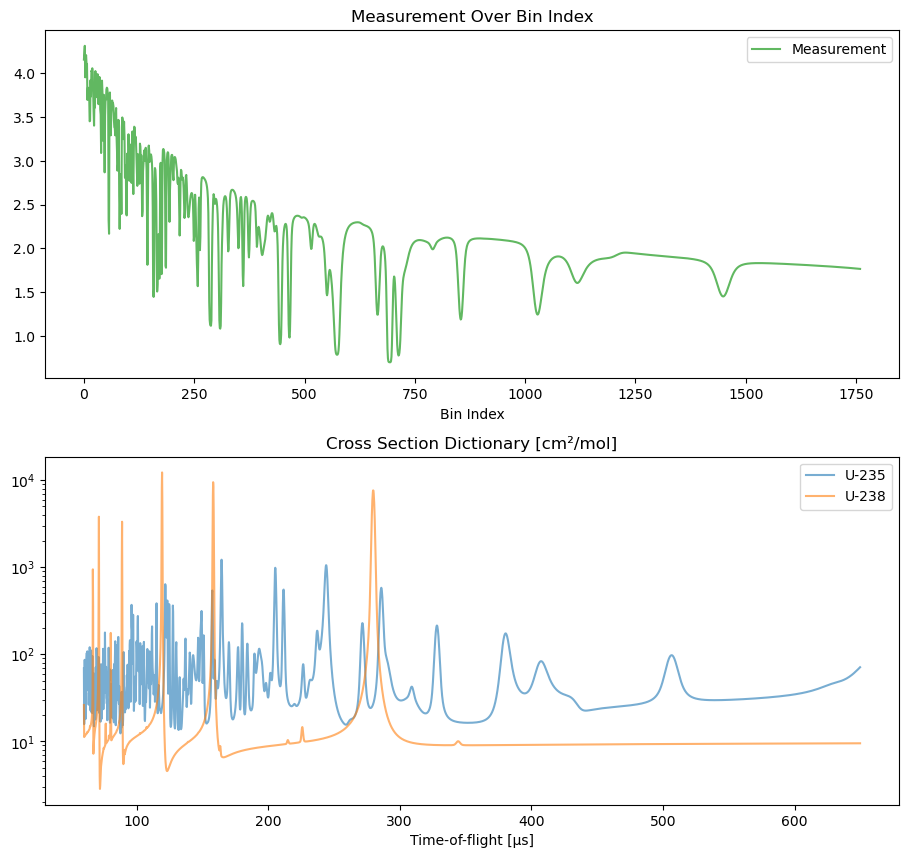
As you can see in the plot above, we only know the bin index for each measurement and we need to find a mapping to TOA.

Since the measurement contains a very distinct cross section profile we can find a few resonances that match the ones found in the plotted cross sections.

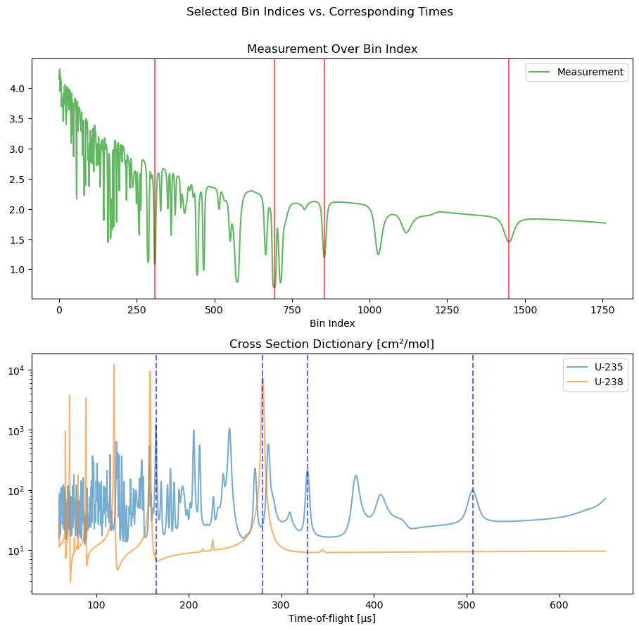
Below we manualy created a list of TOA bin indices and the corresponding TOAs in the cross section dictionary for a few prominent resonances.

bin_index_list = [308.7, 692.9, 854.0, 1448.8]
time_list = [164.6, 279.9, 328.3, 506.6]

We plot the same lines again, highlighting the manually selected values.

fig, ax = plt.subplots(2, 1, figsize=[9, 9], sharex=False)
ax = np.atleast_1d(ax)
ax[0].plot(y_s, label="Measurement", alpha=0.75, color="tab:green")
for x in bin_index_list:
    ax[0].axvline(x=x, c="r", alpha=0.6)
ax[0].set_title("Measurement Over Bin Index")
ax[0].set_xlabel("Bin Index")
ax[0].legend()
D.plot(ax[1])
for x in time_list:
    ax[1].axvline(x=x, c="b", alpha=0.6, ls="--")
fig.suptitle("Selected Bin Indices vs. Corresponding Times")
plt.tight_layout(pad=0.4, w_pad=0.5, h_pad=1.0, rect=(0, 0, 1, 0.95))
plt.show()

Next, we use the following function to find an affine linear mapping from bin index to TOA. The resulting coefficients are the desired values of Δt and t_0.

def bin_number_to_time(bin_index_list, time_list):
    r"""Find affine linear mapping from bin index to time.

    Args:
        bin_index_list: list of bin indices.
        time_list: list of corresponding times.

    Returns:
        The mapping.
    """
    # f(x) = m*x + b
    mb = np.polyfit(bin_index_list, time_list, 1)
    Δt = mb[0]
    t_0 = mb[1]
    return lambda i: Δt * i + t_0


f = bin_number_to_time(bin_index_list, time_list)

The resulting TOA vector is computed below using this mapping.

N_A = y_s.size
t_A = f(np.arange(N_A))  # maps [0, 1, 2, ...] to [t_0, t_1, t_2, ...]

print(f"[{t_A[0] = :.2f}, {t_A[1] = :.2f}, {t_A[2] = :.2f}, ..., {t_A[-1] = :.2f}] μs")

[t_A[0] = 72.05, t_A[1] = 72.35, t_A[2] = 72.65, ..., t_A[-1] = 599.69] μs

Now that the t_A vector is known for the measurements, we can plot the measurements, y_s, and the dictionary, D, on the same x-axis to verify that the calibration was successful.

fig, ax = plt.subplots(1, 1, figsize=[9, 5])
ax = np.atleast_1d(ax)
ax[0].plot(t_A, y_s, label="Measurement", alpha=0.75, color="tab:green")
for x in f(np.array(bin_index_list)):
    ax[0].axvline(x=x, c="r", alpha=0.6)
ax[0].set_xlabel("Time bin index")
ax[0].legend()
D.plot(ax[0])
for x in time_list:
    ax[0].axvline(x=x, c="b", alpha=0.6, ls="--")
ax[0].set_title("Measurement aligned with cross sections")
plt.tight_layout(pad=0.4, w_pad=0.5, h_pad=1.0, rect=(0, 0, 1, 0.95))
plt.show()

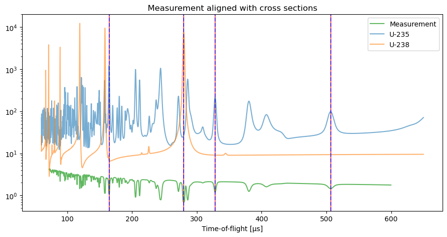
Additionally we can compute the values of Δt and t_0. Note that the estimated values are reltively close to the ground truth values that were printed above.

t_0 = t_A[0]  # = f(0)
Δt = t_A[1] - t_A[0]  # = f(1) - f(0)
print(f"Estitated bin width:        {Δt = :.5f} μs")
print(f"Estitated starting time:    {t_0 = :.2f} μs")

Estitated bin width:        Δt = 0.29997 μs
Estitated starting time:    t_0 = 72.05 μs

If we are interested in the corresponding neutron energies we can use the built-in time2energy function to compute E. Note that by our convention, the t_F (and t_A) arrays are increasing which implies the energy array is decreasing.

E = util.time2energy(t_A, flight_path_length)  # energy array [eV]

print(f"t_A = [{t_A[0]:.2f}, {t_A[1]:.2f}, ..., {t_A[-1]:.2f}] [μs]")
print(f"E   = [{E[0]:.2f}, {E[1]:.2f}, ..., {E[-1]:.2f}] [eV]")

t_A = [72.05, 72.35, ..., 599.69] [μs]
E   = [100.70, 99.87, ..., 1.45] [eV]