[1]:
#!/usr/bin/env python
Demo: trinidi.reconstruct Module#
This script illustrates the functionality of the trinidi.reconstruct submodule.
[2]:
import numpy as np

import matplotlib.pyplot as plt

from trinidi import cross_section, reconstruct, resolution, simulate, util
Generation of Simulated data#
To generate the simulated data we use TRINIDI’s generate_sample_data function that generates a phantom of overlapping discs of different isotopes and the associated measurement counts.
Below we define what isotopes to use for the phantom and what their corresponding densities, z should become. The projection_shape is 2D and is the the size of the detector, but in general it can be of any dimensionality.
[3]:
isotopes = ["U-238", "Pu-239", "Ta-181"]
z = np.array([[0.005, 0.003, 0.004]]).T


# projection_shape = (16, 16) # use this for fast execution
projection_shape = (64, 64)  # use this for the docs

(
    Y_o,
    Y_s,
    ground_truth_params,
    Z,
    t_A,
    flight_path_length,
    N_b,
    kernels,
) = simulate.generate_sample_data(
    isotopes, z, acquisition_time=10, projection_shape=projection_shape
)
The arrays Y_o and Y_s contain the the open beam and sample neutron count measurements. The first (two) axes correspond to projection_shape, which in most cases is equal to the detector shape. The last axis correponds to the time-of-arrival (TOA) dimension which has N_A bins.
[4]:
N_A = Y_o.shape[-1]

print(f"{Y_o.shape = }     (Open beam measurement)")
print(f"{Y_s.shape = }     (Sample measurement)")
print(f"{projection_shape = }     (Shape of the detector)")
print(f"{N_A = }     (Number of TOA bins)")
Y_o.shape = (64, 64, 365)     (Open beam measurement)
Y_s.shape = (64, 64, 365)     (Sample measurement)
projection_shape = (64, 64)     (Shape of the detector)
N_A = 365     (Number of TOA bins)
The corresponding array of TOAs (t_A) is in units of [μs] and has N_A elements.
[5]:
print(f"t_A = [{t_A[0]:.2f}, {t_A[1]:.2f}, ..., {t_A[-2]:.2f}, {t_A[-1]:.2f}] [μs]")
print(f"{t_A.shape = }     (Same as N_A)")
t_A = [72.00, 72.90, ..., 398.70, 399.60] [μs]
t_A.shape = (365,)     (Same as N_A)
The flight_path_length has units of [m] and relates the neutron times with the neutron energies. Below we illustrate the conversion from time to energy.
[6]:
print(f"{flight_path_length = } [m]")
E = util.time2energy(t_A, flight_path_length)
print(f"E = [{E[0]:.2f}, {E[1]:.2f}, ..., {E[-2]:.2f}, {E[-1]:.2f}] [eV]")
flight_path_length = 10 [m]
E = [100.83, 98.36, ..., 3.29, 3.27] [eV]
The ground truth areal densities Z are used in order to later compare to our estimates. Z has the same projection_shape as the measurements. The last axis of Z is the number of isotopes, N_m.
[7]:
N_m = Z.shape[-1]

print(f"{Z.shape = }     (Ground truth areal densities)")
print(f"{N_m = }     (Number of isotopes)")
print(f"{len(isotopes) = }     (Also number of isotopes))")
Z.shape = (64, 64, 3)     (Ground truth areal densities)
N_m = 3     (Number of isotopes)
len(isotopes) = 3     (Also number of isotopes))
We can show the areal densities Z using the plotting function below.
[8]:
def plot_densities(Z, isotopes, vmaxs=None):
    r"""Show areal densities. `ax` must be list."""

    fig, ax = plt.subplots(1, len(isotopes), figsize=[12, 3.3])
    ax = np.atleast_1d(ax)

    for i, isotope in enumerate(isotopes):
        z = Z[:, :, i]
        if vmaxs is None:
            vmax = np.percentile(z, 99.9)
        else:
            vmax = vmaxs[i]
        vmin = 0
        im = ax[i].imshow(z, vmin=vmin, vmax=vmax)
        fig.colorbar(im, ax=ax[i], format="%.1e")
        ax[i].set_title(f"{isotope}")
        ax[i].axis("off")

    fig.suptitle("Areal Densities [mol/cm²]")

    return fig, ax


plot_densities(Z, isotopes, vmaxs=z * 1.5)
plt.show()
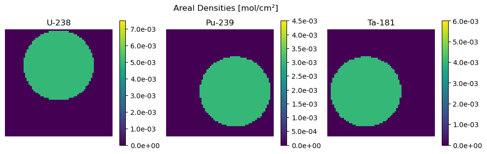
As shown above, the phantom consists of several discs and the ith disc corresponds to isotopes[i] which has density z[i], so it is equal to Z[:,:,i].max().
[9]:
for i, (iso, z_i) in enumerate(zip(isotopes, z.flatten())):
    print(f"{iso}: {z_i} = ({Z[:,:,i].max()}) [mol/cm²]")
U-238: 0.005 = (0.005) [mol/cm²]
Pu-239: 0.003 = (0.003) [mol/cm²]
Ta-181: 0.004 = (0.004) [mol/cm²]
Preparation for the Reconstruction#
For the reconstruction we need to define the regions Ω_z and Ω_0 that correspond to the so called uniformly dense region and the open beam region, respectively.
For this we use the ProjectionRegion class. We initialize each with a mask (boolean array) that has shape projection_shape + (1,), indicating which pixels belong to these regions.
In this example we use the ground truth Z to find these regions as - the overlap of all discs: Ω_z - the complement of the union of all discs: Ω_0.
(In the general case when the ground truth is not known, the user will have to find a way to define these regions such as through prior knowledge about where to adequately find such regions.)
[10]:
mask_z = np.prod(Z, axis=2, keepdims=True) > 0
Ω_z = reconstruct.ProjectionRegion(mask_z)

mask_0 = np.sum(Z, axis=2, keepdims=True) == 0
Ω_0 = reconstruct.ProjectionRegion(mask_0)

print(f"mask_z.shape = mask_0.shape = {mask_0.shape}")
mask_z.shape = mask_0.shape = (64, 64, 1)
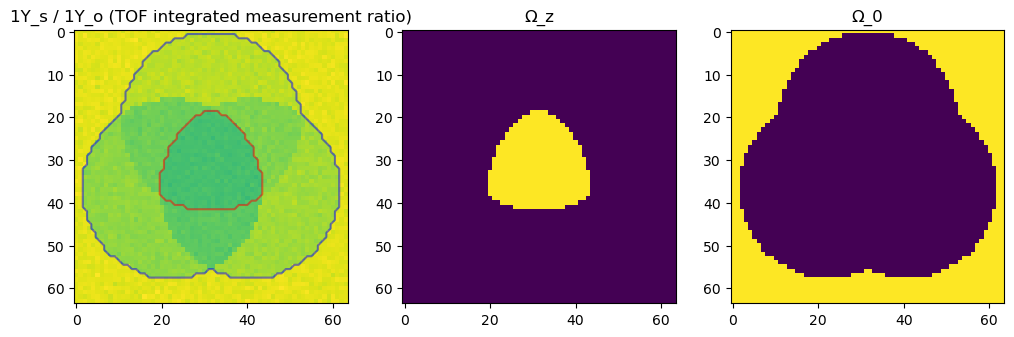
We can illustrate these regions using the ProjectionRegion.plot_contour and the ProjectionRegion.imshow functions below.
[11]:
fig, ax = plt.subplots(1, 3, figsize=[12, 4])
ax = np.atleast_1d(ax)

ax[0].imshow(np.sum(Y_s, axis=-1) / np.sum(Y_o, axis=-1), vmin=0)
ax[0].set_title("1Y_s / 1Y_o (TOF integrated measurement ratio)")
Ω_z.plot_contours(ax[0], color="red")
Ω_0.plot_contours(ax[0], color="blue")

Ω_z.imshow(ax[1], title="Ω_z")
Ω_0.imshow(ax[2], title="Ω_0")

plt.show()
Next we need to define the resolution operator, R. We use the same kernels used for the generation of the data to initialize the ResolutioOperator object.
[12]:
R = resolution.ResolutionOperator(Y_s.shape, t_A, kernels=kernels)
print(R)
<class 'trinidi.resolution.ResolutionOperator'>
    input_shape = (64, 64, 367) = projection_shape + (N_F,)
    output_shape = (64, 64, 365) = projection_shape + (N_A,)

    projection_shape = (64, 64)
    N_F = 367
    N_A = 365
Since the resolution operator inputs wider spectra than it outputs, there is an additional vector of time-of-flights (TOF), t_F, with size N_F, associated with the input times. The t_F array is calibrated such that approximately R(t_A) = t_F.
[13]:
t_F = R.t_F
N_F = t_F.size

print(f"{N_A = }")
print(f"t_A = [{t_A[0]:.2f}, {t_A[1]:.2f}, ..., {t_A[-2]:.2f}, {t_A[-1]:.2f}] [μs]")
print(f"{N_F = }")
print(f"t_F = [{t_F[0]:.2f}, {t_F[1]:.2f}, ..., {t_F[-2]:.2f}, {t_F[-1]:.2f}] [μs]")
N_A = 365
t_A = [72.00, 72.90, ..., 398.70, 399.60] [μs]
N_F = 367
t_F = [71.10, 72.00, ..., 400.05, 400.95] [μs]
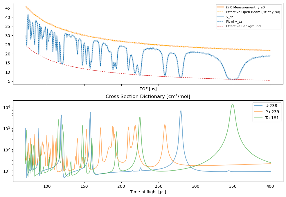
The cross section dictionary uses t_F as calibration for the neutron energies. Below we define the XSDict object.
[14]:
D = cross_section.XSDict(isotopes, t_F, flight_path_length)
print(D)
<class 'trinidi.cross_section.XSDict'>
    isotopes = ['U-238', 'Pu-239', 'Ta-181']
    N_m = 3

    t_F = [71.099 μs, ..., 400.951 μs]
    Δt = 0.901 μs
    N_F = 367
    flight_path_length = 10.000 m
    E = [103.401 eV, ..., 3.251 eV]

    samples_per_bin = 10

    values.shape = (3, 367) = (N_m, N_F)
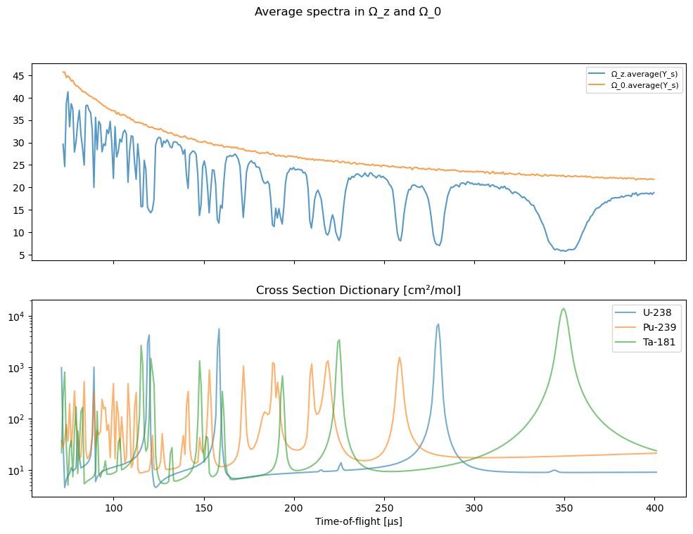
Below we plot the average measurements in the Ω_z and Ω_0 regions compared to the cross section dictionary. We use the ProjectionRegion.averge function to compute these average spectra.
[15]:
fig, ax = plt.subplots(2, 1, figsize=[12, 8], sharex=True)
ax = np.atleast_1d(ax)
ax[0].plot(t_A, Ω_z.average(Y_s).flatten(), label="Ω_z.average(Y_s)", alpha=0.75)
ax[0].plot(t_A, Ω_0.average(Y_s).flatten(), label="Ω_0.average(Y_s)", alpha=0.75)
D.plot(ax[1])
ax[0].legend(prop={"size": 8})
fig.suptitle("Average spectra in Ω_z and Ω_0")
plt.show()
Reconstruction of the Nuisance Parameters#
The nuisance parameters are computed first before the densities can be computed. They parametrize such quantities associated the the neutron flux and background at every pixel (Φ, B) and global scalers such as the overall relative exposure and sample induced background factors (α_1, α_2). We do not expect the general user to need to understand these parameters intricately and thus the handling of these parameters is encapsulated inside the ParameterEstimator object.
Below we define a ParameterEstimator object. For the background we use the same number N_b of basis functions as used for the simulation. This estimates the nuisance parameters (z, α_1, α_1, θ) using the relatively fast BFGS algorithm.
[16]:
par = reconstruct.ParameterEstimator(Y_o, Y_s, R, D, Ω_z, Ω_0=Ω_0, N_b=N_b)
Advanced users: The parameters are available through the ParameterEstimator.get function. They can manually be modified using the ParameterEstimator.set function. We also provide similar save and load functions to write/read them to file.
[17]:
d = par.get()
print(d)


par.set(**d)
par.set(z=d["z"], α_1=d["α_1"], α_2=d["α_2"], θ=d["θ"])  # same as line above

# par.save("par.npy")
# d = par.load("par.npy")
{'z': array([[0.00499364],
       [0.00298873],
       [0.00398788]]), 'α_1': 1.199791365376037, 'α_2': 0.7998832057418127, 'θ': array([[46.73438273],
       [-8.81218864],
       [ 0.35045738]])}
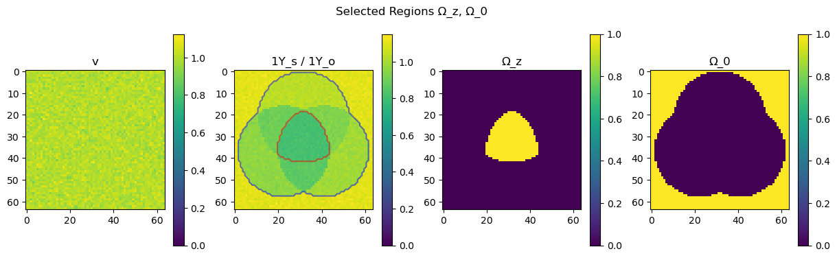
Once the ParameterEstimator object has been constructed we can plot the Ω_z and Ω_0 regions much more easily than above using the ParameterEstimator.plot_regions function.
[18]:
par.plot_regions()
plt.show()
The ParameterEstimator.plot_results function allows to display the resulting spectra from the estimation and verify good fitting of the signals.
[19]:
par.plot_results()
plt.show()
We also provide the APGM optimization routine used in our paper, however we do not recommend it since tends to be signicicantly slower.
[20]:
# par.apgm_solve(iterations=100)
# fig, ax = par.apgm_plot_convergence(plot_residual=True, ground_truth=ground_truth_params)
# plt.show()
Reconstruction of the Areal Densities#
Now that the nuisance parameters have been computed and stored in the ParameterEstimator object, we can carry on with the main task, i.e. with the areal density reconstruction.
We define a DensityEstimator object. Note that if the optional arguments D and R are left empty, the D and R operators from the par Parameters object will be used for the reconstruction.
(If different D and R operators are desired, they need to be passed to the DensityEstimator constructor.)
[21]:
den = reconstruct.DensityEstimator(Y_s, par, non_negative_Z=False, dispperiod=50)
We reonstruct the areal densities using the DensityEstimator.solve function which returns the areal density estimates Z_hat.
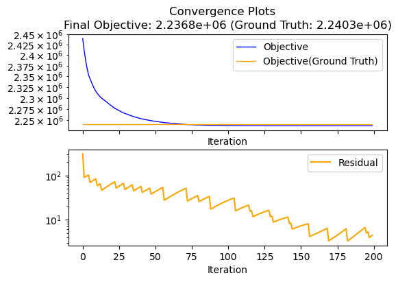
[22]:
Z_hat = den.solve(iterations=200)
Iter  Time      Objective  L          Residual
-----------------------------------------------
   0  6.39e+00  2.440e+06  4.719e+00  3.068e+02
  50  1.77e+01  2.247e+06  6.226e+00  4.319e+01
 100  2.88e+01  2.237e+06  4.107e+00  2.742e+01
 150  4.00e+01  2.237e+06  5.418e+00  7.244e+00
 199  5.11e+01  2.237e+06  7.943e+00  4.426e+00
We can plot the convergence of the objective using the DensityEstimator.plot_convergence function. The ground truth argument is optional and will additionaly display the objective to the ground truth.
[23]:
den.plot_convergence(ground_truth=Z)
plt.show()
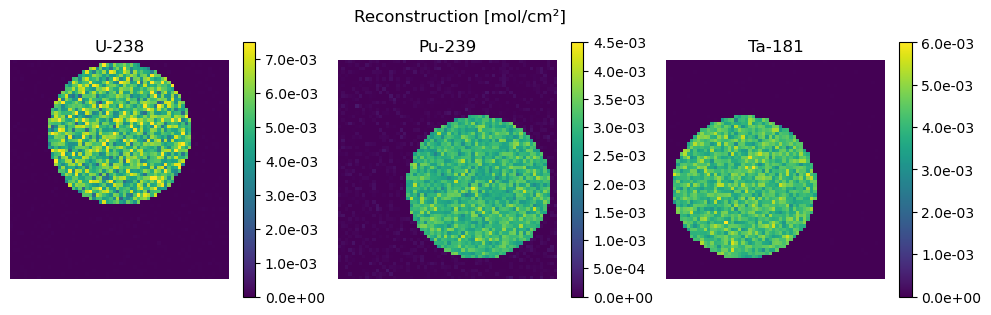
We use this plotting function below to plot the resulting areal density estimates and compare them to the ground truth (Z)
[24]:
def plot_compare(Z, str_Z, Z_hat, str_Z_hat):
    r"""Generate two plots comparing ground truth with reconstruction."""
    fig, ax = plot_densities(Z, isotopes, vmaxs=z * 1.5)
    fig.suptitle(f"{str_Z} [mol/cm²]")

    fig, ax = plot_densities(Z_hat, isotopes, vmaxs=z * 1.5)
    fig.suptitle(f"{str_Z_hat} [mol/cm²]")


plot_compare(Z, "Ground Truth", Z_hat, "Reconstruction")
plt.show()

Cropped or Binned Measurements#
In practice, it is not always desired to reconstruct the full field of view or at full resolution: Perhaps we require the full field of view to estimate the nuisance parameters, but we only want to reconstruct a small cropped region. For this reason we can provide the projection_transform argument in the DensityEstimator constructor.
The projection_transform is the desired operation that is applied to the measurements and used internally to handle the modification of the background and flux estimates.
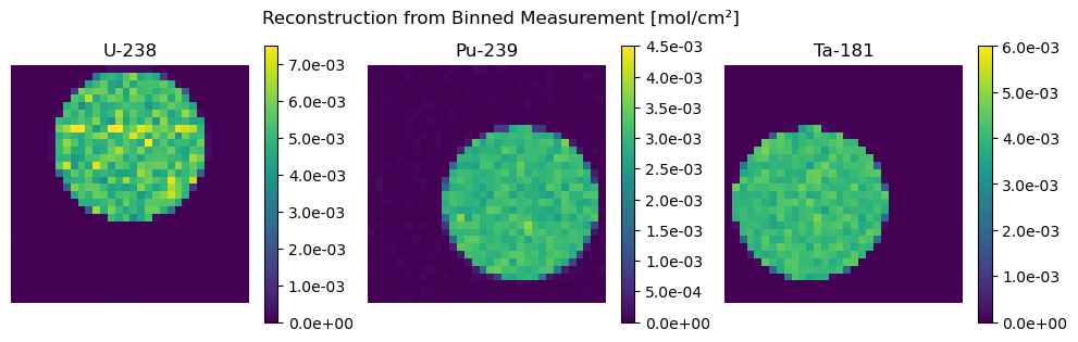
First we show an example of binned data using the below defined binning_2x2 function.
[25]:
def binning_2x2(Y):
    r"""Bin an array of shape (N, M, ...) with the result being (N//2, M//2, ...)"""
    N0 = Y.shape[0] // 2
    N1 = Y.shape[1] // 2
    Y = Y[0::2][:N0] + Y[1::2][:N0]
    Y = Y[:, 0::2][:, :N1] + Y[:, 1::2][:, :N1]
    return Y
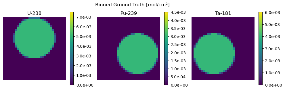
We define the DensityEstimator but pass the binning_2x2 as the projection_transform argument and use solve as usual. Note that the resulting detector shape is half the size in each direction.
[26]:
den = reconstruct.DensityEstimator(
    Y_s, par, projection_transform=binning_2x2, non_negative_Z=False, dispperiod=50
)
den.solve(iterations=200)

Z_binned = binning_2x2(Z) / (2 * 2)  # over 4 to keep ground truth scale the same.
Z_hat_binned = den.Z

print(f"{Z.shape = }")
print(f"{Z_binned.shape = }")
Iter  Time      Objective  L          Residual
-----------------------------------------------
   0  2.17e+00  8.868e+05  1.887e+01  1.511e+02
  50  4.98e+00  6.986e+05  2.490e+01  2.001e+01
 100  7.67e+00  6.914e+05  3.286e+01  7.198e+00
 150  1.03e+01  6.915e+05  1.084e+01  2.789e+00
 199  1.29e+01  6.913e+05  1.589e+01  3.242e+00
Z.shape = (64, 64, 3)
Z_binned.shape = (32, 32, 3)
We plot the results below.
[27]:
plot_compare(
    Z_binned, "Binned Ground Truth", Z_hat_binned, "Reconstruction from Binned Measurement"
)
plt.show()
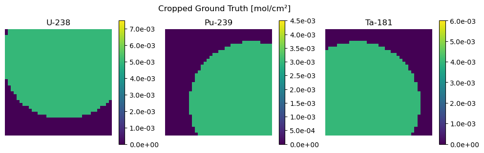
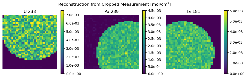
Second we show an example of cropping data using the below defined crop function.
[28]:
def crop(Y):
    r"""Create center crop from 1/5 to 4/5 of the FOV."""
    N0 = Y.shape[0] // 5
    N1 = Y.shape[1] // 5
    Y = Y[N0 : 4 * N0, N1 : 4 * N1]
    return Y


den = reconstruct.DensityEstimator(
    Y_s, par, projection_transform=crop, non_negative_Z=False, dispperiod=50
)
den.solve(iterations=200)

Z_crop = crop(Z)
Z_hat_crop = den.Z

print(f"{Z_crop.shape = }")
print(f"{Z.shape = }")


plot_compare(Z_crop, "Cropped Ground Truth", Z_hat_crop, "Reconstruction from Cropped Measurement")
plt.show()
Iter  Time      Objective  L          Residual
-----------------------------------------------
   0  2.46e+00  8.261e+05  4.719e+00  2.451e+02
  50  5.69e+00  6.987e+05  3.113e+00  4.956e+01
 100  8.97e+00  6.925e+05  4.107e+00  1.917e+01
 150  1.22e+01  6.925e+05  5.418e+00  4.378e+00
 199  1.55e+01  6.924e+05  7.943e+00  3.773e+00
Z_crop.shape = (36, 36, 3)
Z.shape = (64, 64, 3)
If multiple transformations are required, those can easily be composed such as below.
[29]:
projection_transform = lambda Y: crop(binning_2x2(Y))