#!/usr/bin/env python

Demo: trinidi.resolution Module

This script illustrates the functionality of the trinidi.resolution submodule.

import numpy as np

import matplotlib.pyplot as plt

from trinidi import cross_section, resolution, util

Overview

The resolution operator, \(R\), models the uncertainty distribution of the emission time of the neutrons. In the idealized case, when the neutron pulse is instantaneous, the time-of-arrival (TOA) is equal to the time-of-flight (TOF) and the resolution operator is equal to the identity: \(R = I\). However, in practice the neutron pulse often has a significant durantion and match the TOA (i.e. the measured time at the detector plane) does not deterministically the TOF (i.e. the neutron energy).

If \(Z\) is the array of areal densities and \(D\) is the cross section dictionary, then the expected transmission \(Q\) is

\[Q = \exp (-ZD) R = Q_0 R\;.\]

In this script we will generate artificial raw transmission data, \(Q_0\), and the resolution operator \(R\) to generate the blurred transmission spectrum \(Q = Q_0 R\). We define the blurred transmission spectrum to correspond to the TOA sampling vector \(t_A\) and the raw transmission to correspond the the TOF sampling vector, \(t_F\). The \(t_A\) samples are a subset of the \(t_F\) samples so that boundary effects due to the blurring are avoided.

Defining the TOA sampling vector

By our convention, the \(t_A\) vector has equidistant and increasing sampling.

Δt = 0.30  # bin size in μs
t_A = np.arange(72, 450, Δt)
N_A = t_A.size  # number of TOA bins

The corresponding energy range of the neutrons is computed and displayed below. Note that the corresponding energy samples are neither equidistant nor increasing.

flight_path_length = 10  # flight path length in m

E = util.time2energy(t_A, flight_path_length)

print(f"t_A = [{t_A[0]:.3f}, {t_A[1]:.3f}, ..., {t_A[-1]:.3f}] μs")
print(f"E = [{E[-1]:.3f}, {E[-2]:.3f}, ..., {E[0]:.3f}] eV")

t_A = [72.000, 72.300, ..., 449.700] μs
E = [2.585, 2.588, ..., 100.830] eV

Defining the Output Shape

When defining the resolution operator, the output_shape of the operator must be passed to the constructor. The output_shape is equal to projection_shape + (N_A,) where projection_shape is usually the size of the detector.

projection_shape = (3, 3)
output_shape = projection_shape + (N_A,)

Defining a Resolution Operator

In this example we use a set of primitive rectangular convolution kernels. The t_F TOF sampling vector is retrieved from R and in general it is larger than t_A.

kernels = [np.ones(10) / 10, np.ones(20) / 20, np.ones(30) / 30]
R = resolution.ResolutionOperator(output_shape, t_A, kernels=kernels)
t_F = R.t_F  # the TOF sampling vector
N_F = t_F.size

print(f"t_A = [{t_A[0]:.3f}, {t_A[1]:.3f}, ..., {t_A[-1]:.3f}] μs")
print(f"t_F = [{t_F[0]:.3f}, {t_F[1]:.3f}, ..., {t_F[-1]:.3f}] μs")

print(f"{N_F = } ≥ {N_A = }")

t_A = [72.000, 72.300, ..., 449.700] μs
t_F = [69.450, 69.750, ..., 454.050] μs
N_F = 1283 ≥ N_A = 1260

We can display the resolution operator attributes like this:

print(R)

<class 'trinidi.resolution.ResolutionOperator'>
    input_shape = (3, 3, 1283) = projection_shape + (N_F,)
    output_shape = (3, 3, 1260) = projection_shape + (N_A,)

    projection_shape = (3, 3)
    N_F = 1283
    N_A = 1260

Next, we can apply the resolution operator to a synthetic transmission spectrum.

Below we define a cross section dictionary, D, using the t_F sampling vector. The areal densities, Z are equal to z.T at every pixel.

isotopes = ["Pu-239", "U-235"]
N_M = len(isotopes)  # number of isotopes

z = np.array([[1e-3], [2e-3]])  # areal density in mol/cm²
Z = np.ones(projection_shape + (1,)) @ z.T  # 2D areal density map
print(f"{Z[0,0] = } [mol/cm²]")  # printing first pixel areal densities


D = cross_section.XSDict(isotopes, t_F, flight_path_length)  # cross section in cm²/mol

Z[0,0] = array([0.001, 0.002]) [mol/cm²]

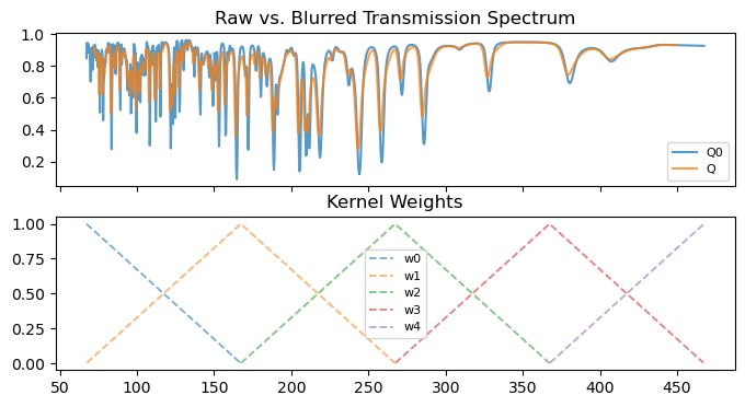
The synthetic raw spectrum, Q0, and the blurred spectrum Q are computed and plotted below. We also plot the associated weights that indicate at which TOF which kernels are active.

Q0 = np.exp(-Z @ D.values)
Q = R(Q0)

fig, ax = plt.subplots(2, 1, figsize=[8, 4], sharex=True)
ax = np.atleast_1d(ax)
ax[0].plot(t_F, Q0[0, 0], label="Q0", alpha=0.75)
ax[0].plot(t_A, Q[0, 0], label="Q", alpha=0.75)
ax[0].legend(prop={"size": 8})
ax[0].set_title("Raw vs. Blurred Transmission Spectrum")
R.plot_kernel_weights(ax[1])

plt.show()

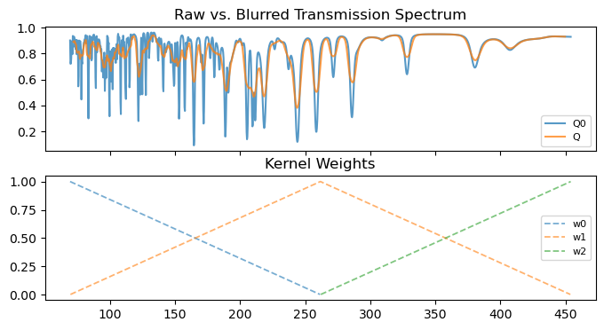
Defining a General Resolution Operator

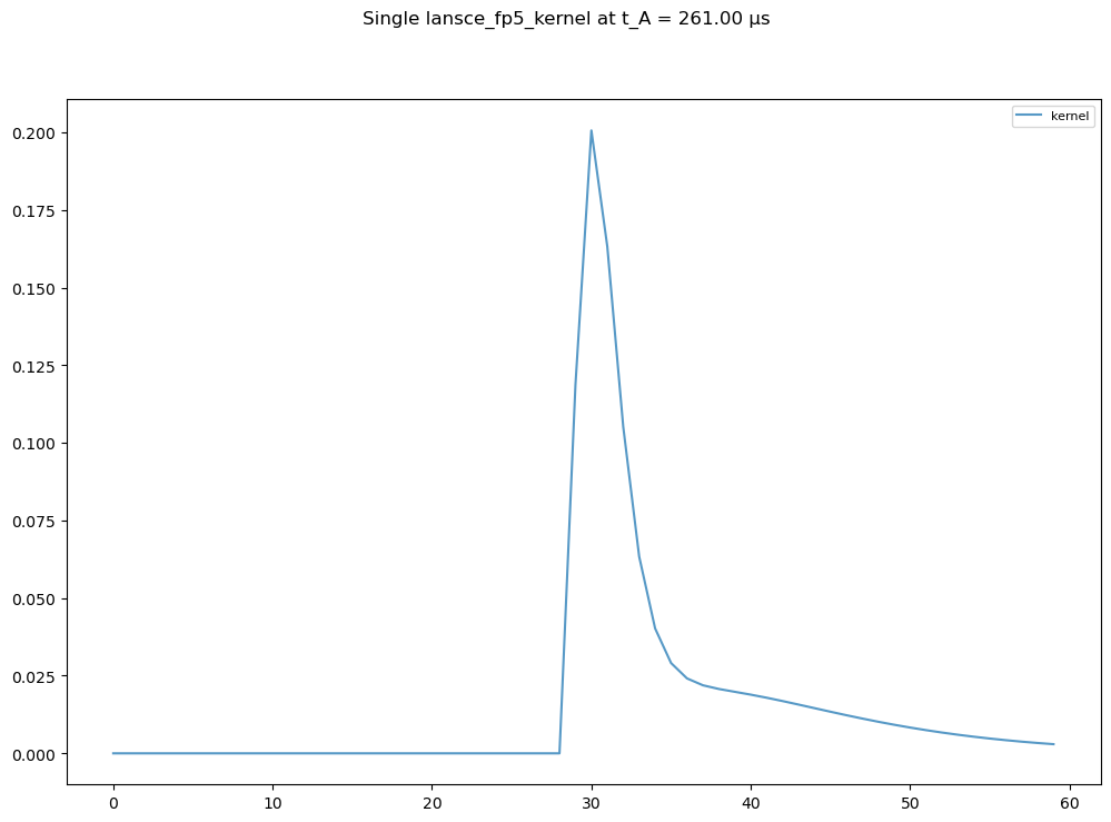
If we have a function that computes the blurring kernel as a function of TOA, below we show how we can create the corresponding kernels. We illustrate this using the built-in lansce_fp5_kernel function and the equispaced_kernels function.

The lansce_fp5_kernel function computes the kernel shape as a function of TOA and other parameters for a particular flight path facility. Below we generate the kernel at the center TOA.

i = N_A // 2  # center index
kernel = resolution.lansce_fp5_kernel(t_A[i], Δt, flight_path_length)


fig, ax = plt.subplots(1, 1, figsize=[12, 8], sharex=True)
ax = np.atleast_1d(ax)
ax[0].plot(kernel, label="kernel", alpha=0.75)
ax[0].legend(prop={"size": 8})
fig.suptitle(f"Single lansce_fp5_kernel at t_A = {t_A[i]:.2f} μs")
# plt.savefig('')
plt.show()

For the resolution operator we require these kernels at equispaced TOAs. First we need a function g with a single argument, t_A.

# i.e. g(t_A) == resolution.lansce_fp5_kernel(t_A, Δt, flight_path_length)
g = lambda t_A: resolution.lansce_fp5_kernel(t_A, Δt, flight_path_length)

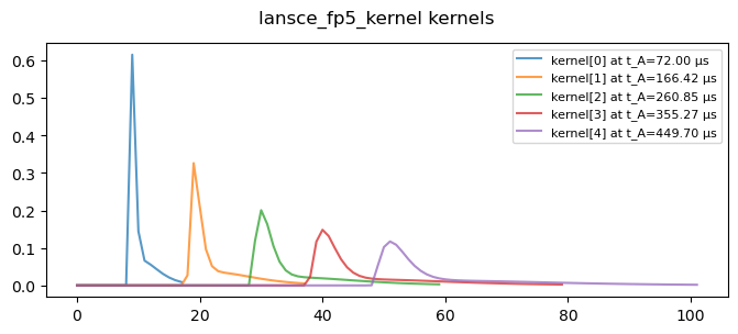
The equispaced_kernels function generates the appropriate kernels.

num_kernels = 5
kernels, t_As = resolution.equispaced_kernels(t_A, num_kernels, g)

fig, ax = plt.subplots(1, 1, figsize=[8, 3], sharex=True)
ax = np.atleast_1d(ax)
for i, kernel in enumerate(kernels):
    ax[0].plot(kernel, label=f"kernel[{i}] at t_A={t_As[i]:.2f} μs", alpha=0.75)
ax[0].legend(prop={"size": 8})
fig.suptitle(f"lansce_fp5_kernel kernels")
# plt.savefig('')
plt.show()

Below we show the resulting synthetic spectra.

R = resolution.ResolutionOperator(output_shape, t_A, kernels=kernels)
t_F = R.t_F

D = cross_section.XSDict(isotopes, t_F, flight_path_length)  # cross section in cm²/mol


Q0 = np.exp(-Z @ D.values)
Q = R(Q0)

fig, ax = plt.subplots(2, 1, figsize=[8, 4], sharex=True)
ax = np.atleast_1d(ax)
ax[0].plot(t_F, Q0[0, 0], label="Q0", alpha=0.75)
ax[0].plot(t_A, Q[0, 0], label="Q", alpha=0.75)
ax[0].legend(prop={"size": 8})
ax[0].set_title("Raw vs. Blurred Transmission Spectrum")
R.plot_kernel_weights(ax[1])

plt.show()

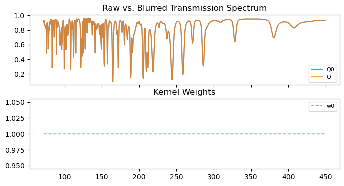
Identity Resolution Operator

If it is desired to omit the resolution operator, you can simply create an identity resolution operator setting the kernels=None argument.

R = resolution.ResolutionOperator(output_shape, t_A, kernels=None)
t_F = R.t_F
N_F = t_F.size

Note: This is equivalent to using a single dirac kernel:

print(R.kernels)

[array([1])]

Only in the case of the identity operator the TOF and TOA sampling vectors are equal to each other and have the same length, i.e. R is a square linear operator.

if np.allclose(t_F, t_A) and (N_F == N_A):
    print("t_F == t_A")
    print(f"N_F == N_A == {N_A}")

t_F == t_A
N_F == N_A == 1260

Below we show the resulting synthetic spectra (which are of course equal).

D = cross_section.XSDict(isotopes, t_F, flight_path_length)  # cross section in cm²/mol


Q0 = np.exp(-Z @ D.values)
Q = R(Q0)

fig, ax = plt.subplots(2, 1, figsize=[8, 4], sharex=True)
ax = np.atleast_1d(ax)
ax[0].plot(t_F, Q0[0, 0], label="Q0", alpha=0.75)
ax[0].plot(t_A, Q[0, 0], label="Q", alpha=0.75)
ax[0].legend(prop={"size": 8})
ax[0].set_title("Raw vs. Blurred Transmission Spectrum")
R.plot_kernel_weights(ax[1])

plt.show()