#!/usr/bin/env python

Demo: trinidi.cross_section Module

This script illustrates the functionality of the trinidi.cross_section submodule.

from copy import deepcopy

import numpy as np

import matplotlib.pyplot as plt

from trinidi import cross_section

Available Isotopes

First we demonstrate how to display available isotopes and display their energy ranges.

The cross_section.info function prints out info for all isotopes.

# cross_section.info() # Uncomment this line to print the complete output.

# H-1       10.0 µeV to 20.0 MeV
# H-2       10.0 µeV to 150.0 MeV
# H-3       10.0 µeV to 20.0 MeV
# He-3      10.0 µeV to 20.0 MeV
# He-4      10.0 µeV to 20.0 MeV
# Li-6      10.0 µeV to 20.0 MeV
# Li-7      10.0 µeV to 20.0 MeV
# Be-7      10.0 µeV to 20.0 MeV
# Be-9      10.0 µeV to 20.0 MeV
# B-11      10.0 µeV to 20.0 MeV
# C-12      10.0 µeV to 150.0 MeV
# .
# .
# .

We access a list of all available isotopes using the cross_section.avail function.

av_isotopes = cross_section.avail()
print(
    f"av_isotopes = [{av_isotopes[0]}, {av_isotopes[1]}, ..., {av_isotopes[-2]}, {av_isotopes[-1]}]"
)
print(f"Number of isotopes = {len(av_isotopes)}")

av_isotopes = [H-1, H-2, ..., Es-255, Fm-255]
Number of isotopes = 533

You can restrict the displayed isotopes by cross_section.info using the isotopes optional argument. Below we subselect all the uranium isotopes.

isotopes_U = [iso for iso in av_isotopes if iso.split("-")[0] == "U"]
print("\nUranium Isotopes:")
cross_section.info(isotopes=isotopes_U)

Uranium Isotopes:
U-230   10.0 µeV to 20.0 MeV
U-231   10.0 µeV to 20.0 MeV
U-232   10.0 µeV to 20.0 MeV
U-233   10.0 µeV to 20.0 MeV
U-234   10.0 µeV to 30.0 MeV
U-235   10.0 µeV to 30.0 MeV
U-236   10.0 µeV to 30.0 MeV
U-237   10.0 µeV to 30.0 MeV
U-238   10.0 µeV to 30.0 MeV
U-239   10.0 µeV to 30.0 MeV
U-240   10.0 µeV to 30.0 MeV
U-241   10.0 µeV to 30.0 MeV

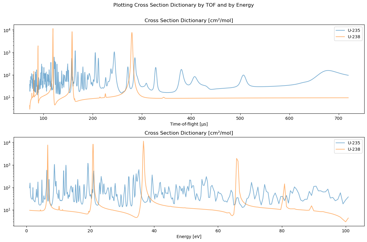
Generate and Plot a Cross Section Dictionary Object XSDict

First we setup the time-of-flight (TOF) array and requested isotopes list. Note that the cross section dictionary is sampled with equispaced samples in TOF.

Δt = 0.30  # bin width [μs]
flight_path_length = 10  # [m]
t_F = np.arange(72, 720, Δt)  # time-of-flight array [μs]
isotopes = ["U-235", "U-238"]

Create a XSDict cross section dictionary object.

D = cross_section.XSDict(isotopes, t_F, flight_path_length)
print(D)

<class 'trinidi.cross_section.XSDict'>
    isotopes = ['U-235', 'U-238']
    N_m = 2

    t_F = [72.000 μs, ..., 719.700 μs]
    Δt = 0.300 μs
    N_F = 2160
    flight_path_length = 10.000 m
    E = [100.830 eV, ..., 1.009 eV]

    samples_per_bin = 10

    values.shape = (2, 2160) = (N_m, N_F)

The np.ndarray D.values is a matrix of size N_m x N_F that contains the cross section values.

print(f"{D.values.shape = }")

D.values.shape = (2, 2160)

You can plot the dictionary easily with the XSDict.plot function. The optional argument function_of_energy=False [default] allows plotting it as a function of time-of-flight while function_of_energy=True plots it as a function of energy.

fig, ax = plt.subplots(2, 1, figsize=[12, 8], sharex=False)
ax = np.atleast_1d(ax)
D.plot(ax[0])
D.plot(ax[1], function_of_energy=True)
fig.suptitle("Plotting Cross Section Dictionary by TOF and by Energy")
plt.tight_layout(pad=0.4, w_pad=0.5, h_pad=1.0, rect=(0, 0, 1, 0.95))
plt.show()

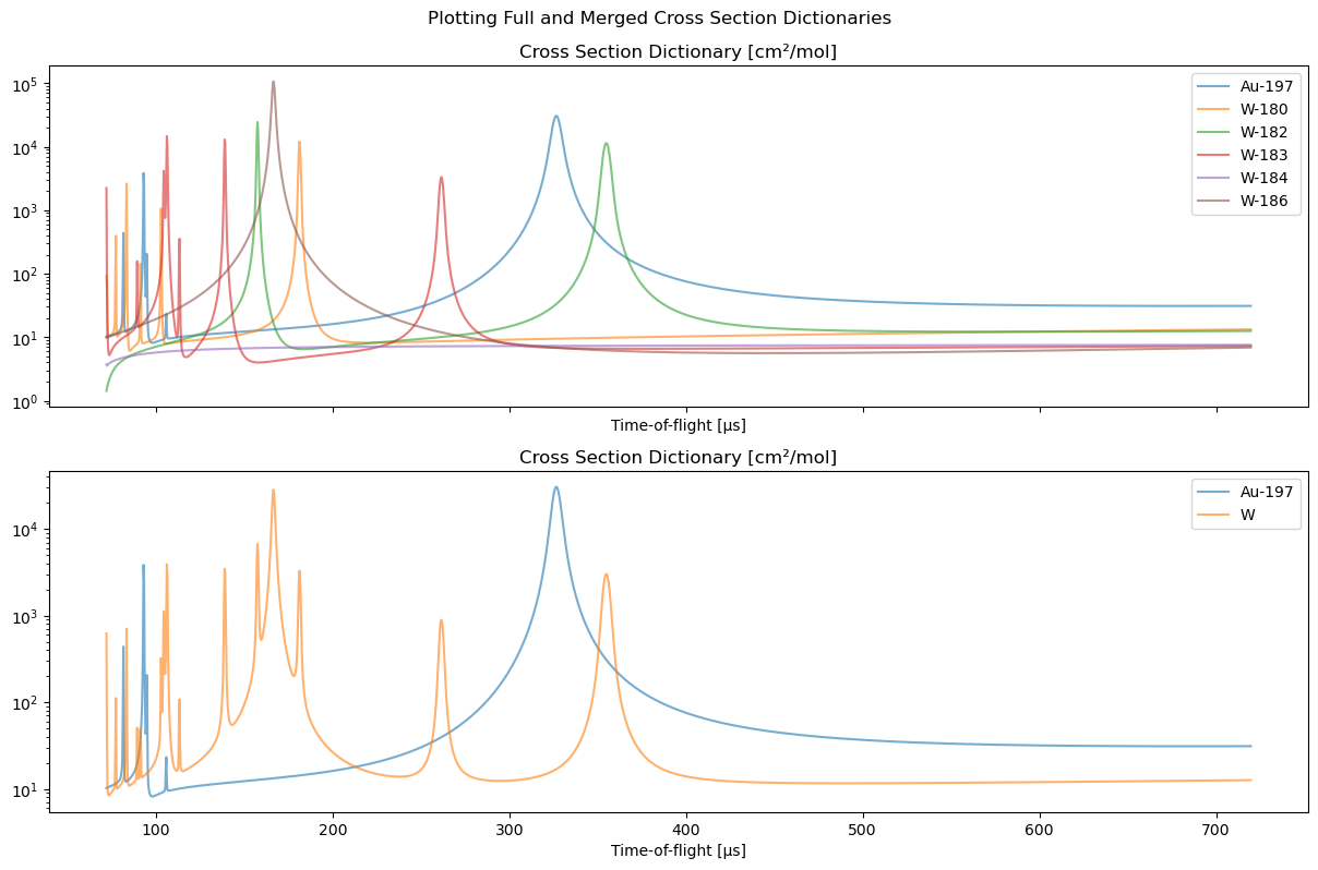
Creating a Compound Material Cross Section Dictionary

When reconstructing a sample with isotopes in known proportions, we recommend combining the corresponding isotopes according to their known abundances and treating it as a compound material.

For example, below we show how we construct a gold and tungsten (Au, W) cross section dictionary. Gold is practically 100% Au-197 so no action is necessary. However, elemental tungsten consists of several isotopes,

# W-180: 0.12%
# W-182: 26.5%
# W-183: 14.3%
# W-184: 30.6%
# W-186: 28.4%

which we want to combine into a single entry with the use of the XSDict.merge function.

We start out with the XSDict using all isotopes. The D_full object will stay untouched and used for later comparison.

isotopes_full = ["Au-197", "W-180", "W-182", "W-183", "W-184", "W-186"]
D_full = cross_section.XSDict(isotopes_full, t_F, flight_path_length)

We now define the arguments for the XSDict.merge function. The arguments below result in a new cross section that will be

\[\sigma_{\mathrm{W}} = 0.0012 \times \sigma_{\mathrm{W180}} + \dots + 0.284 \times \sigma_{\mathrm{W186}}\]

and a new dictionary that will be

\[D_{\mathrm{new}} = [\sigma_{\mathrm{Au197}}, \sigma_{\mathrm{W}}]^\top\]

merge_isotopes = ["W-180", "W-182", "W-183", "W-184", "W-186"]
merge_weights = [0.0012, 0.265, 0.143, 0.306, 0.284]
new_key = "W"

Below, we generate the modified XSDict object, D_new from a copy of D_full.

D_new = deepcopy(D_full)
isotopes_new = D_new.merge(merge_isotopes, merge_weights, new_key)
print(f"New isotope list: {isotopes_new}")
print(D_new)

New isotope list: ['Au-197', 'W']
<class 'trinidi.cross_section.XSDict'>
    isotopes = ['Au-197', 'W']
    N_m = 2

    t_F = [72.000 μs, ..., 719.700 μs]
    Δt = 0.300 μs
    N_F = 2160
    flight_path_length = 10.000 m
    E = [100.830 eV, ..., 1.009 eV]

    samples_per_bin = 10

    values.shape = (2, 2160) = (N_m, N_F)

The merge_isotopes cross sections are combined using a weighted sum using the merge_weights. All previous isotope keys, ["W-180", "W-182", "W-183", "W-184", "W-186"], will be replaced by the new_key, "W", which is defined by the user.

(Note that the updated list XSDict.isotopes is now not necessarily strictly isotopes since "W" is not an isotope. After creation this list primarily serves for plotting and identification of the entries.)

Below we plot and compare the resulting XSDict objects.

fig, ax = plt.subplots(2, 1, figsize=[12, 8], sharex=True)
ax = np.atleast_1d(ax)
D_full.plot(ax[0])
D_new.plot(ax[1])
plt.tight_layout(pad=0.4, w_pad=0.5, h_pad=1.0, rect=(0, 0, 1, 0.95))
fig.suptitle("Plotting Full and Merged Cross Section Dictionaries")
plt.show()